Материал: Damage Propagation Modeling

Abstract— This paper describes how damage propagation can be modeled within the modules of aircraft gas turbine engines. To that end, response surfaces of all sensors are generated via a thermo-dynamical simulation model for the engine as a function of variations of flow and efficiency of the modules of interest. An exponential rate of change for flow and efficiency loss was imposed for each data set, starting at a randomly chosen initial deterioration set point. The rate of change of the flow and efficiency denotes an otherwise unspecified fault with increasingly worsening effect. The rates of change of the faults were constrained to an upper threshold but were otherwise chosen randomly. Damage propagation was allowed to continue until a failure criterion was reached. A health index was defined as the minimum of several superimposed operational margins at any given time instant and the failure criterion is reached when health index reaches zero. Output of the model was the time series (cycles) of sensed measurements typically available from aircraft gas turbine engines. The data generated were used as challenge data for the Prognostics and Health Management (PHM) data competition at PHM’08.

Index Terms—Damage modeling, Prognostics, C-MAPSS, Turbofan engines, Performance Evaluation

CONTENTS

I.Introduction………….………………………. 1

II.Prognostics………….…………………..…… 1

III.System Model……………………..…………. 2

V.Application Scenario …………………….…... 5

Manuscript received May 18, 2008. This work was supported in part by the U.S. National Aeronautics and Space Administration (NASA) under the Integrated Vehicle Health Management (IVHM) program.

Abhinav Saxena, is with Research Institute for Advanced Computer Science at NASA Ames Research Center, Moffett Field, CA 94035 USA (Phone: 650-604-3208; fax: 650-604-4036; e-mail: asaxena@mail.arc.nasa.gov).

Kai Goebel is with NASA Ames Research Center, Moffett Field, CA 94035 USA.

Don Simon is with NASA Glenn Research Center, Cleveland, OH, 44135 USA.

Neil Eklund is with GE Global Research, Niskayuna, NY 12309

I. INTRODUCTION

Data-driven prognostics faces the perennial challenge of the lack of run-to-failure data sets. In most cases realworld data contain fault signatures for a growing fault but no or little data capture fault evolution until failure. Procuring actual system fault progression data is typically time consuming and expensive. Fielded systems are, most of the time, not properly instrumented for collection of relevant data. Those fortunate enough to be able to collect long-term data for fleets of systems tend to – understandably – hold the data from public release for proprietary or competitive reasons. Few public data repositories (e.g., [1]) exist that make run-to-failure data available. The lack of common data sets, which researchers can use to compare their approaches, is impeding progress in the field of prognostics. While several forecasting competitions have been held in the past (e.g., [2-7]), none have been conducted with a PHM-centric focus. All this provided the motivation to conduct the first PHM data challenge. The task was to estimate remaining life of an unspecified system using historical data only,

irrespective of the underlying physical process.

For most complex systems like aircraft engines, finding a suitable model that allows the injection of health related changes certainly is a challenge in itself. In addition, the question of how the damage propagation should be modeled within a model needed to be addressed. Secondary issues revolved around how this propagation would be manifested in sensor signatures such that users could build meaningful prognostic solutions.

In this paper we first define the prognostics problem to set the context. Then the following sections introduce the simulation model chosen, along with a brief review of health parameter modeling. This is followed by a description of the damage propagation modeling, a description of the competition data, and a discussion on performance evaluation.

II. PROGNOSTICS

To avoid confusion, we define prognostics here exclusively as the estimation of remaining useful component life. The remaining useful life (RUL) estimates are in units of time (e.g., hours or cycles). End-of-life can be subjectively determined as a function of operational

thresholds that can be measured. These thresholds depend on user specifications to determine safe operational limits.

Prognostics is currently at the core of systems health management. Reliably estimating remaining life holds the promise for considerable cost savings (for example by avoiding unscheduled maintenance and by increasing equipment usage) and operational safety improvements. Remaining life estimates provide decision makers with information that allows them to change operational characteristics (such as load) which in turn may prolong the life of the component. It also allows planners to account for upcoming maintenance and set in motion a logistics process that supports a smooth transition from faulty equipment to fully functional. Aircraft engines (both military and commercial), medical equipment, power plants, etc. are some of the common examples of these types of equipment.

Therefore, it is not surprising that finding solutions to the prognostics problem is a very active research area. The fact that most efforts are focusing on data-driven approaches seems to reflect the desire to harvest low-hanging fruit as compared to model-based approaches, irrespective of the difficulties in gaining an access to statistically significant amounts of run-to-failure data and common metrics that allow a comparison between different approaches.

Next we will describe how a system model can be used to generate run-to-failure data that can then be utilized to develop, train, and test prognostic algorithms.

III. SYSTEM MODEL

Tracking and predicting the progression of damage in aircraft engine turbo machinery has some roots in the work of Kurosaki et al. [8]. They estimate the efficiency and the flow rate deviation of the compressor and the turbine based on operational data, and utilize this information for fault detection purposes. Further investigations have been done by Chatterjee and Litt on on-line tracking and accommodating engine performance degradation effects represented by flow capacity and efficiency adjustments [9]. In [10], response surfaces for various sensors outputs are generated for a range of flow and efficiency values using a simulation model. These response surfaces are used to identify flow and efficiency health parameters of an actual engine by optimally matching the set of sensor readings with simulated sensor values, resulting in only one possible solution. The process chosen here continues on a similar path and follows closely the one described in [10].

An important requirement for the damage modeling process was the availability of a suitable system model that allows input variations of health related parameters and recording of the resulting output sensor measurements. The recently released C-MAPSS (Commercial Modular AeroPropulsion System Simulation) [11] meets these requirements and was chosen for this work.

A. C-MAPSS

C-MAPSS is a tool for simulating a realistic large

commercial turbofan engine. The software is coded in the MATLAB® and Simulink® environment, and includes a number of editable input parameters that allow the user to enter specific values of his/her own choice regarding operational profile, closed-loop controllers, environmental conditions, etc. C-MAPSS simulates an engine model of the 90,000 lb thrust class and the package includes an atmospheric model capable of simulating operations at (i) altitudes ranging from sea level to 40,000 ft, (ii) Mach numbers from 0 to 0.90, and (iii) sea-level temperatures from –60 to 103 °F. The package also includes a powermanagement system that allows the engine to be operated over a wide range of thrust levels throughout the full range of flight conditions.

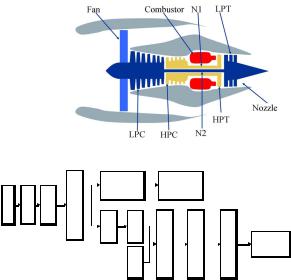
In addition, the built-in control system consists of a fanspeed controller, and a set of regulators and limiters. The latter include three high-limit regulators that prevent the engine from exceeding its design limits for core speed, engine-pressure ratio, and High-Pressure Turbine (HPT) exit temperature; a limit regulator that prevents the static pressure at the High-Pressure Compressor (HPC) exit from going too low; and an acceleration and deceleration limiter for the core speed. A comprehensive logic structure integrates these control-system components in a manner similar to that used in real engine controllers such that integrator-windup problems are avoided. Furthermore, all of the gains for the fan-speed controller and the four limit regulators are scheduled such that the controller and regulators perform as intended over the full range of flight conditions and power levels. The engine diagram in Figure 1 shows the main elements of the engine model and the flow chart in Figure 2 shows how various subroutines are assembled in the simulation.

Figure 1. Simplified diagram of engine simulated in C-MAPSS [11].

Nozzle

Figure 2. A layout showing various modules and their connections as modeled in the simulation [11].

CMAPSS can be operated either in open-loop (without any controller) or in closed loop (with the engine and its control system) configurations. For the purpose of this

paper, we worked exclusively with the closed-loop configuration. C-MAPSS has 14 inputs (Table 1) and can produce several outputs. Table 2 lists the outputs that were used for the challenge data. The inputs include fuel flow and a set of 13 health-parameter inputs that allow the user to simulate the effects of faults and deterioration in any of the engine’s five rotating components (Fan, LPC, HPC, HPT, and LPT). The outputs include various sensor response surfaces and operability margins. A total of 21 variables out of 58 different outputs available from the model were used in this study. C-MAPSS provides a set of Graphical User Interfaces (GUIs) to simplify input and output control for a variety of possible uses, including open-loop analysis, controller-design, and simulation of response of the engine and its control system in a variety of situations. However, for the purpose of this data generation exercise, we ran the model in batch-mode without using the GUIs.

Table 1. C-MAPSS inputs to simulate various degradation scenarios in any of the five rotating components of the simulated engine. For example, to simulate HPC degradation HPC flow and efficiency modifiers were used (highlighted in gray).

Table 2. C-MAPSS outputs to measure system response. Margins were used for health index calculation only and were not available to the participants explicitly.

B. Response Surfaces

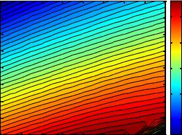
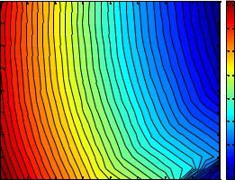
To ensure that the output of the model was producing correct results, we first generated response surfaces for sensed outputs and operability margins from C-MAPSS as a function of flow and efficiency for specific modules. These were compared with those published by Goebel et al. [10]. Although it was not expected that the units would match (in fact, none were revealed in [10]), it was expected that the qualitative response should be similar. For instance, with an increase in flow and efficiency, the response surface behaved in a similar fashion as obtained from the real aircraft engine used in [10]. For each module in the gas path (HPC, HPT, and LPT), the efficiencies and flows were incrementally changed and C-MAPSS was then run under different cruise conditions randomly chosen at each time step. Some resulting HPC module response surfaces for the high pressure compressor stall margin and the exhaust gas temperature (EGT) are shown in Figure 3 and Figure 4, respectively.

Efficiency Loss (%)

Figure 3. Response surface of HPC stall margin as a function of efficiency and flow losses simulating degradation in HPC module.

The range of the flow and efficiency loss is the same in all figures. Response surfaces for the other modules’ sensors and operability margins were also generated using the same process and verified.

Efficiency Loss (%)

Figure 4. Response surface for Exhaust Gas Temperature (EGT) as a function of efficiency and flow losses.

IV. DAMAGE PROPAGATION MODELING

Having decided on the system model, the next hurdle is to model the propagation of damage. Common models used across different application domains include the Arrhenius model, the Coffin-Manson mechanical crack growth model, and the Eyring model (for more than three stresses or when the above models are not satisfactory) [12]. These models come in numerous variations that will not be discussed here.

A. Arrhenius

The Arrhenius model has been used for a variety of failure mechanisms. Traditionally, it has been applied to those that depend on chemical reactions, diffusion processes or migration processes. While this covers many of the nonmechanical (or non-material fatigue) failure modes that cause electronic equipment failure, lately, variations of the Arrhenius equation have also been employed for mechanical and other non-traditional applications. The operative equation is:

A is a scaling factor,

f is the cycling frequency,

T is the temperature range during a cycle,

G(Tmax) is an Arrhenius term evaluated at the maximum temperature reached in each cycle,

α is the cycling frequency exponent, and

βis the temperature range exponent.

C. Eyring Model

The Eyring Model originates in chemical reaction rate theory and has a theoretical basis in chemistry and quantum mechanics. It describes how time to failure varies with stress. The base model includes temperature and can be expanded to include other relevant stresses. The temperature term by itself is very similar to the Arrhenius empirical model, explaining why that model has been so successful in establishing the connection between the H parameter and the quantum theory concept of "activation energy needed to cross an energy barrier and initiate a reaction".

The model for temperature and additional stress terms takes the general form:

where

tf is the time to failure,

α, H, A, B, C, D, and E are constants that determine acceleration between stress combinations,

S1 and S2 are relevant stresses (e.g., some function of voltage or current),

T is temperature in degrees Kelvin, and k is the Boltzmann’s constant.

The general Eyring model includes terms that have stress and temperature interactions. A disadvantage of the Eyring model is that it has a relatively large number of parameters that need to be determined.

zero initial degradation, d, (allowing the data-generation process to start at an arbitrary point in the wear-space) which will be modeled as an additive term to yield

The health index can be used to model different phenomena within a subsystem. Specifically, for aircraft engine modules like the compressor and turbine sections, the health is described both by efficiency (e) and flow (f). Trajectories for flow and efficiency vary for different fault modes [4] and are modeled as separate health related indices

The terms e(t) and f(t) are then aggregated to form the overall health index H(t), the engine simulation response to

where, the function g is the minimum of all operative margins considered (here those for fan, HPC, HPT, and

where, the margins m in turn are functions of efficiency e(t) and flow f(t). Calculation of the health index is further discussed in section V.D

V. APPLICATION SCENARIO

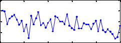
The scenario developed for the challenge data tracks a number of aircraft engines throughout their usage history. A particular engine unit may be employed under different flight conditions from one flight to another. Depending on various factors the amount and rate of damage accumulation will be different for each engine. It is assumed that the amount of damage accumulated during a particular flight will not be directly quantifiable solely based on flight duration and flight conditions, and hence, one must rely on information extracted from sensor data collected during each flight. This scenario models engine performance degradation due to wear and tear based on the usage pattern of the engines and not necessarily due to any particular fault mode. Therefore, sudden degradation during a flight is rather unlikely. This allows us to take one measurement snapshot per flight to characterize the engine health during or right after that flight. Further, the effects of between-flight maintenance have not been explicitly modeled but have been incorporated as the process noise. This allows the engine performance parameters (flow and efficiency) to improve within allowable limits at any point and hence the loss in efficiency or flow is not locally monotonic (see Figure 5).

In order to simulate the scenario explained above we needed to address several issues in order to make it more realistic. Some of these issues and their resolutions are discussed next.

Change in Efficiency Parameter for one Engine

Figure 5. Performance parameters like efficiency and flow may not change monotonically to model process noise that also incorporates between flight maintenance operations, which may lead to improved performance in subsequent flights.

A. Initial Wear

Initial wear can occur due to manufacturing inefficiencies and are commonly observed in real systems. Although it is not considered abnormal, it can make a difference in useful operational life of a component. Initial wear can also be modeled by variations in flow and efficiencies of the various modules, although the magnitude of such variations is relatively low. Chatterjee and Litt [9] give examples for the degree of wear that an engine might experience with progressive usage. These numbers were used as reference values for the challenge data and are recited in Table 3 for reference.

Table 3. Engine wear as manifested in flow and efficiency changes [9].

B. Noise

Characterizing noise in a system may be a non-trivial undertaking. Of various sources, the main sources of noise while assessing the true state of system’s health are manufacturing and assembly variations, process noise (due to factors not taken in to account while modeling the process), and measurement noise to name a few important ones. These noise sources introduce their respective contributions at different stages of the process and a combined effect is observed in the sensor measurements at the end. A simple approach to model this combined effect is to use approximate models (e.g. random noise models) [13, 14]. In other cases sophisticated noise model identification techniques may be employed [15] if real data are available for such analyses. In both situations a PHM practitioner is faced with characterizing and de-noising tasks before