Материал: Damage Propagation Modeling

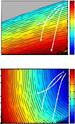
Depending on the direction of the failure evolution trajectory (simulated by changing e and f parameters) a threshold may or may not be crossed. Therefore, the overall health index is determined by the margin that approaches the corresponding limit first. For instance, in the following figures, health index is determined by increasing EGT (decreasing EGT margin) as compared to HPC stall margin for all three degradation trajectories. Each degradation trajectory was simulated until the health index reached zero.

Figure 7. Fault propagation trajectories on HPC stall margin contour map.

Figure 8. Fault propagation trajectories on EGT contour map with failure threshold.

VI. COMPETITION DATA

The objective was to generate train, test, and validation data sets for development of data-driven prognostics. To that end, a reasonably large number of trajectories were created from C-MAPSS that had the following properties:

1)Simulation of degradation in HPC module under 6 different combinations of Altitude, TRA, and Mach number operational conditions. Sensed margins (fan, HPC, LPC and EGT) were used to compute health index to determine simulation stopping criteria.

2)Time series of observables including operational variables (see Table 1 and Table 2), that change from some undefined initial condition to a failure threshold. Participants were not given access to the health index explicitly and were expected to infer it from the given sensed variables.

3)Division of data into training set, test set, and validation

set. The training set had trajectories that ended at the failure threshold while the test and validation sets were pruned to stop some time prior to the failure threshold.

4)The range of RUL variation was expanded for the validation set to test robustness of the algorithms trained on test data set (a condition that was not announced to the participants). The test data set RULs ranged between 10 and 150 cycles, whereas validation RULs ranged between 6 and 190 cycles. However, all other

characteristics like variation in initial wear, noise levels and degradation parameters spread remained changed.

Participants of the challenge were then given details of the scoring function. They could submit their test set results in vector form through a web site where scores were automatically calculated and posted back to the participants, allowing them to improve their algorithms. To avoid overfitting to the test data, the validation set was withheld and published later, without feedback of the score until after the competition had closed.

VII. PERFORMANCE EVALUATION

Performance evaluation is concerned with employing metrics that help assess if the prognosis meets specifications for the task at hand. In PHM context, since the key aspect is to avoid failures, it is generally desirable to predict early as compared to predicting late. However, in specific situations where failures may not pose life threatening situations and early predictions may instead involve significant economic burden, this equation may change and one may not prefer conservative predictions. Hence, a performance evaluation system should reflect such characteristics to meet specific requirements.

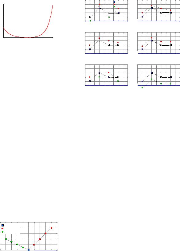
For an engine degradation scenario an early prediction is preferred over late predictions. Therefore, the scoring algorithm for this challenge was asymmetric around the true time of failure such that late predictions were more heavily penalized than early predictions. In either case, the penalty grows exponentially with increasing error. The asymmetric preference is controlled by parameters a1 and a2 in the scoring function given below (eq. 11) and Figure 9 shows the score as a function of the error.

where

s is the computed score, n is the number of UUTs,

d = tˆRUL − tRUL (Estimated RUL – True RUL), a1 = 10, and a2 = 13.

Figure 9. Score as a function of error.

Asymmetric scoring functions like this capture the preference for early prediction pretty well and can be appropriately tuned to quantify the extent of such preference.

While evaluating the results, it was realized that this prognostics metric can be further enhanced in various ways. It must be noted that predicting farther into the future is more difficult than predicting at a time closer to the end of life. Furthermore, it is more important to weigh accuracy of RULs higher when one is closer to the end of life. Keeping these thoughts in mind it may be desirable to assign higher weights for cases with shorter true RULs. Another characteristic of such datasets is that the performance of an algorithm is evaluated from multiple units under test (UUTs), e.g., in fleet applications. Since the metric is a combined aggregate of performance for individual UUTs, an additional correlation metric should be employed to ensure that an algorithm consistently predicts well for all cases as against predicting well for some and poorly for the rest. This idea is illustrated in Figure 10 and Figure 11 shows a simplified asymmetric scoring function used for this illustration.

The various axes shown in Figure 11 show six different cases of prognostics algorithm outputs. Each axis shows estimated RULs and the corresponding true RULs for four UUTs. A simple asymmetric function (see Figure 10) is used to compute scores from RUL predictions for each UUT. As shown, each of these six cases produces an equal aggregated score of six. Clearly one can further differentiate in the output performance based on the suggested correlation metric. In some applications a higher correlation score may be preferred over lower aggregated scores, as a higher correlation may indicate a bias in the algorithm output that can be accordingly adjusted.

Prediction Error

Figure 10. A simplified asymmetric scoring function chosen for illustration

Figure 11. Scenarios illustrating various cases where error based aggregated scores may be same but the correlation score distinguishes further between different algorithms.

These suggestions are just to illustrate the point that there may be more modifications possible depending on specific applications and requirements and one must adapt accordingly. A comprehensive review of prognostics metrics is given in [20].

VIII. CONCLUSION

This paper has described how damage propagation can be modeled in various modules of aircraft gas turbine engines for developing and testing prognostics algorithms. A publically available aero-propulsion system simulator, C- MAPSS, was used in this study. Various assumptions and settings have been provided that were used to generate data for the PHM competition at the first international conference on prognostics and health management. Although, the data for the competition consisted of a subset of various possible conditions and settings, an insight into other possibilities can be easily derived. Later, a brief discussion has been provided on the performance evaluation of prognostics algorithms and the aspects of the performance metrics that may be desirable in a PHM application.

ACKNOWLEDGEMENTS

The authors would like to thank Dean Frederick for providing valuable insight into the operation of C-MAPSS.

REFERENCES

[1]NASA, "Prognostics Center of Excellence Data Repository", http://ti.arc.nasa.gov/projects/data_prognostics, last accessed on January, 2007.

[2]H. Madsen, G. Kariniotakis, H. A. Nielsen, T. S. Nielsen, and P. Pinson, "A Protocol for Standardizing the Performance Evaluation of Short-Term Wind Power Prediction Models,"