Документ: AD620, страницы 6-10

AD620–Typical Characteristics

1000

fA/!Hz





–
NOISECURRENT	100
	100
	10

1	10	100	1000
		FREQUENCY – Hz
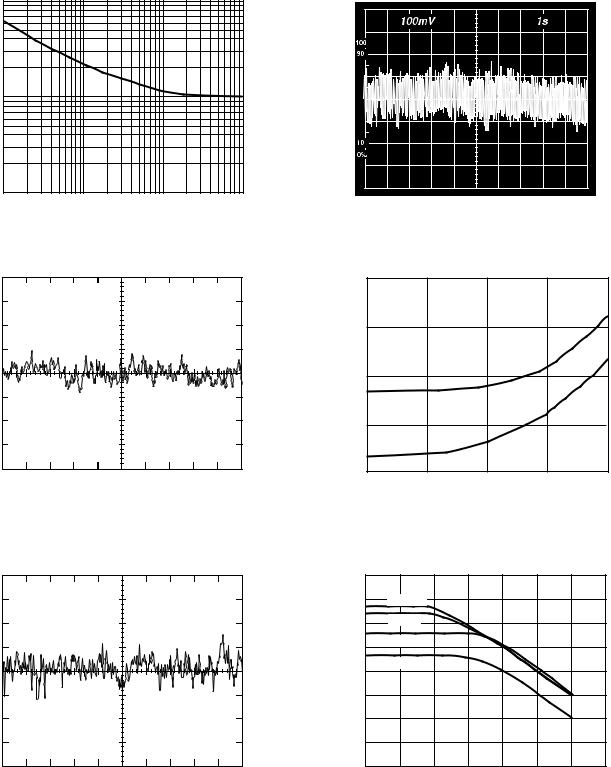
Figure 9. Current Noise Spectral Density vs. Frequency				Figure 11. 0.1 Hz to 10 Hz Current Noise, 5 pA/Div

	100,000
	–mV
	RTI	10,000
2.0mV/DIV	CTO 858C,	10,000
2.0mV/DIV	CTO 858C,				IN-AMP
					FET INPUT
NOISE –	FROM 258	1000
NOISE –	FROM 258
RTI	DRIFT					AD620A
						AD620A
		100
	TOTAL
TIME – 1 SEC/DIV		10	10k	100k	1M	10M
TIME – 1 SEC/DIV		1k	10k	100k	1M	10M
				SOURCE RESISTANCE –V

Figure 10a. 0.1 Hz to 10 Hz RTI Voltage Noise (G = 1)

Figure 12. Total Drift vs. Source Resistance

0.1mV/DIV

RTI NOISE –

TIME – 1 SEC/DIV

Figure 10b. 0.1 Hz to 10 Hz RTI Voltage Noise (G = 1000)

	+160
	+140	G = 1000
	+120	G = 100
	+120
	+100	G = 10
dB	+100
dB		G = 1
–	+80	G = 1
–
CMR
CMR	+60
	+60
	+40
	+20
	0		10	100	1k	10k	100k
	0.1	1	10	100	1k	10k	100k	1M
				FREQUENCY – Hz

Figure 13. CMR vs. Frequency, RTI, Zero to 1 kΩ Source Imbalance

–6–

REV. E

												AD620
180									35
										G = 10, 100, 1000
160									30
								p-p	30
140								p-p
140					G = 1000			Volts	25
					G = 1000				25
120
120								OUTPUTVOLTAGE –		G = 1
									20
100						G = 100
80									15	BW LIMIT
80
						G = 10			10
60									10
60
dB–PSR
40						G = 1			5
40									5	G = 1000
										G = 1000	G = 100
											G = 100
20									0
0.1	1	10	100	1k	10k	100k	1M		1k	10k	100k	1M

FREQUENCY – Hz	FREQUENCY – Hz
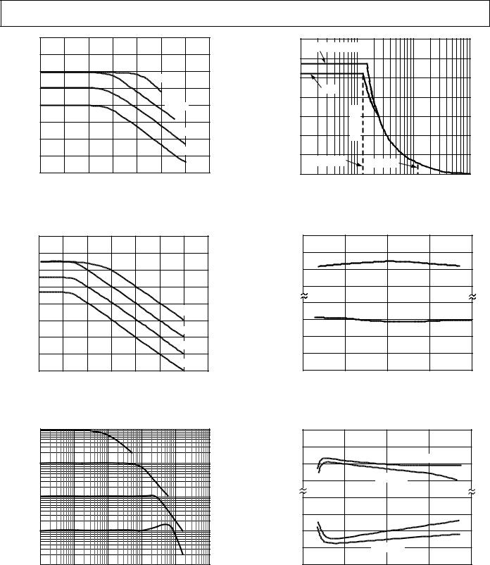
Figure 14. Positive PSR vs. Frequency, RTI (G = 1–1000)	Figure 17. Large Signal Frequency Response

	180
	160
	140
	120
– dB	100
PSR							G = 1000
PSR	80
	80
							G = 100
	60
							G = 10
	40
	20						G = 1
	20
	0.1	1	10	100	1k	10k	100k	1M
				FREQUENCY – Hz

Figure 15. Negative PSR vs. Frequency, RTI (G = 1–1000)

1000

100

V/V– 10

GAIN

1

0.1	1k	10k	100k	1M	10M
100

FREQUENCY – Hz

		+VS –0.0
	(REFERRED TO SUPPLY VOLTAGES)	–0.5
INPUT VOLTAGE LIMIT – Volts		–1.0
		–1.5
		+1.5
		+1.0
		+0.5
		+0.5
		–V +0.0
		S	5	10	15	20
		0	5	10	15	20

SUPPLY VOLTAGE 6 Volts

Figure 18. Input Voltage Range vs. Supply Voltage, G = 1

	+VS –0.0
OUTPUT VOLTAGE SWING – Volts	(REFERRED TO SUPPLY VOLTAGES)	–0.5
		–1.0			RL = 10kV
		–1.0
		–1.5		RL = 2kV
		–1.5
		+1.5
				RL = 2kV
		+1.0
		+0.5		RL = 10kV
	–V	+0.0
	S	0	5	10	15	20
		0	5	10	15	20

SUPPLY VOLTAGE 6 Volts

Figure 16. Gain vs. Frequency	Figure 19. Output Voltage Swing vs. Supply Voltage,
	G = 10

REV. E

–7–

AD620

p-p	30
	30

Volts		G = 10
		VS = 615V
–	20


SWING
SWING
VOLTAGEOUTPUT	10
	10
	0
	0
	0	100		1k	10k
			LOAD RESISTANCE –V

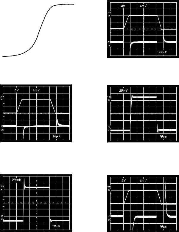
Figure 20. Output Voltage Swing vs. Load Resistance

. . . . . . . . . . . . . . . . . . . . . . . . . . . . . . . . . . . . . . . .

Figure 23. Large Signal Response and Settling Time, G = 10 (0.5 mV = 001%)

. . . . . . . . . . . . . . . . . . . . . . . . . . . . . . . . . . . . . . . .

Figure 21. Large Signal Pulse Response and Settling Time G = 1 (0.5 mV = 0.01%)

Figure 24. Small Signal Response, G = 10, RL = 2 kΩ, CL = 100 pF

. . . . . . . . . . . . . . . . . . . . . . . . . . . . . . . . . . . . . . . .

Figure 22. Small Signal Response, G = 1, RL = 2 kΩ, CL = 100 pF

Figure 25. Large Signal Response and Settling Time, G = 100 (0.5 mV = 0.01%)

–8–

REV. E

						AD620
		20
. . . . . . . . . . . . . . . . . . . . . . . . . . . . . . . . . . . . . . . .		15
		15		TO 0.01%
	–ms			TO 0.01%
	–ms					TO 0.1%
	TIME	10
	SETTLING	10
	SETTLING
. . . . . . . . . . . . . . . . . . . . . . . . . . . . . . . . . . . . . . . .		5

		0	5	10	15	20
		0	5	10	15	20

OUTPUT STEP SIZE – Volts

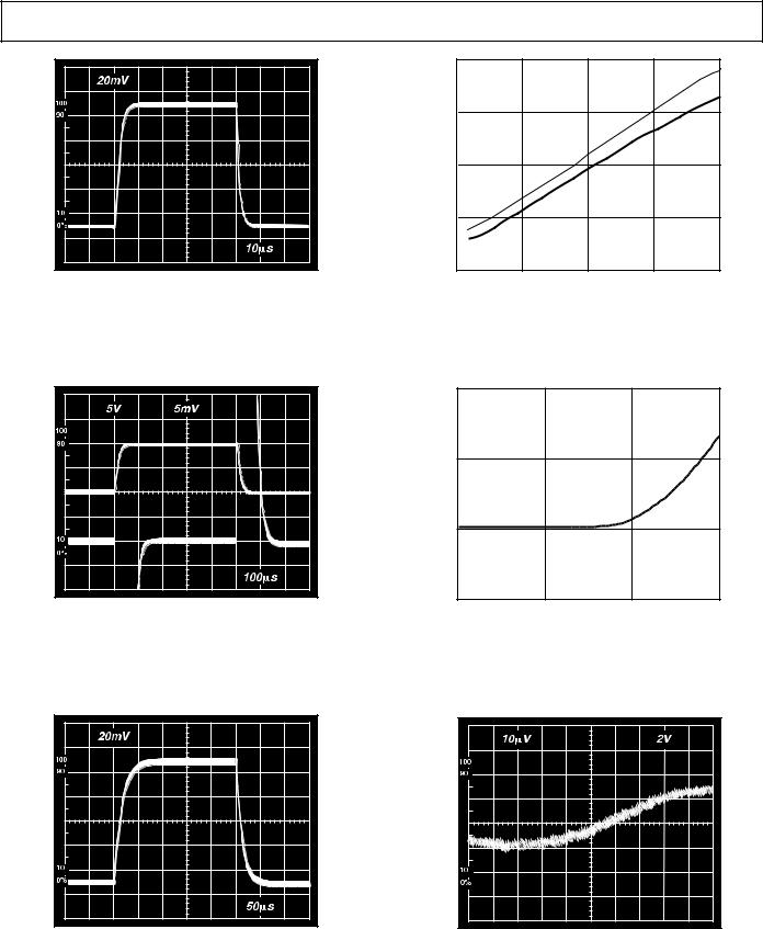
Figure 26. Small Signal Pulse Response, G = 100, RL = 2 kΩ, CL = 100 pF

Figure 29. Settling Time vs. Step Size (G = 1)

. . . . . . . . . . . . . . . . . . . . . . . . . . . . . . . . . . . . . . . .

Figure 27. Large Signal Response and Settling Time, G = 1000 (0.5 mV = 0.01%)

. . . . . . . . . . . . . . . . . . . . . . . . . . . . . . . . . . . . . . . .

Figure 28. Small Signal Pulse Response, G = 1000, RL = 2 kΩ, CL = 100 pF

	1000
s
–m	100
–m
SETTLING TIME	10
	1
	1	10	100	1000
			GAIN

Figure 30. Settling Time to 0.01% vs. Gain, for a 10 V Step

. . . . . . . . . . . . . . . . . . . . . . . . . . . . . . . . . . . . . . . .

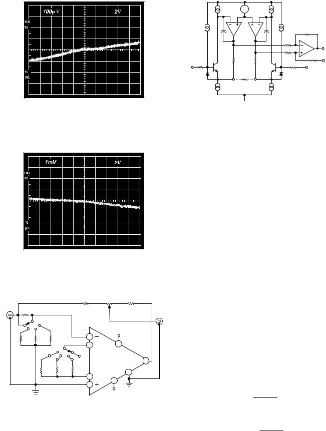
Figure 31a. Gain Nonlinearity, G = 1, RL = 10 kΩ

(10 μV = 1 ppm)

REV. E

–9–

AD620

. . . . . . . . . . . . . . . . . . . . . . . . . . . . . . . . . . . . . . . .

Figure 31b. Gain Nonlinearity, G = 100, RL = 10 kΩ

(100 μV = 10 ppm)

. . . . . . . . . . . . . . . . . . . . . . . . . . . . . . . . . . . . . . . .

Figure 31c. Gain Nonlinearity, G = 1000, RL = 10 kΩ
(1 mV = 100 ppm)
			10kV*	1kV	10kV
INPUT			10kV*	10T	10kV
INPUT
10V p-p
100kV					VOUT
					VOUT
				+VS
11kV	1kV	100V	2
11kV	1kV	100V
			1	7
	G=1000		G=1
		G=100	G=10	AD620	6
		G=100
	49.9V 499V		5.49kV		5
			8		5
			8	4
			3	4
			3
				–V
				S
*ALL RESISTORS 1% TOLERANCE

Figure 32. Settling Time Test Circuit

I1	20mA	VB	20mA	I2
	A1		A2		10kV
					10kV
	C1		C2
				10kV
					A3	OUTPUT
R3	R1		R2	10kV	10kV	REF
R3
400V
400V
– IN	Q1			Q2	+IN
		RG		R4
		RG		400V
	GAIN		GAIN
	SENSE		SENSE
		–V
		S

Figure 33. Simplified Schematic of AD620

THEORY OF OPERATION

The AD620 is a monolithic instrumentation amplifier based on a modification of the classic three op amp approach. Absolute value trimming allows the user to program gain accurately (to 0.15% at G = 100) with only one resistor. Monolithic construction and laser wafer trimming allow the tight matching and tracking of circuit components, thus ensuring the high level of performance inherent in this circuit.

The input transistors Q1 and Q2 provide a single differentialpair bipolar input for high precision (Figure 33), yet offer 10¥ lower Input Bias Current thanks to Superbeta processing. Feedback through the Q1-A1-R1 loop and the Q2-A2-R2 loop maintains constant collector current of the input devices Q1, Q2 thereby impressing the input voltage across the external gain setting resistor RG. This creates a differential gain from the inputs to the A1/A2 outputs given by G = (R1 + R2)/RG + 1. The unity-gain subtracter A3 removes any common-mode signal, yielding a single-ended output referred to the REF pin potential.

The value of RG also determines the transconductance of the preamp stage. As RG is reduced for larger gains, the transconductance increases asymptotically to that of the input transistors. This has three important advantages: (a) Open-loop gain is boosted for increasing programmed gain, thus reducing gainrelated errors. (b) The gain-bandwidth product (determined by C1, C2 and the preamp transconductance) increases with programmed gain, thus optimizing frequency response. (c) The input voltage noise is reduced to a value of 9 nV/ÖHz, determined mainly by the collector current and base resistance of the input devices.

The internal gain resistors, R1 and R2, are trimmed to an absolute value of 24.7 kW, allowing the gain to be programmed accurately with a single external resistor.

The gain equation is then

= 49.4 kW +

G 1

RG so that

= 49.4 kW

RG G - 1

–10–

REV. E

Материал: AD620

Смотрите также: