Материал: Russian Journal of Building Construction and Architecture

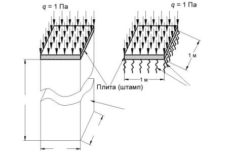
sized 1 1 m, height 10 m (the distance from the bottom of the shell to the bottom of the massive from the section above, i.e. the depth of the compressed soil) loaded at the top with the pressure 1 Pа transmitted onto the massive with the stiff stamp (Ешт = 2 1015 Pа, = 0.3). The massive (Fig. 3а) is supported not to be shifted towards the normal along the sides and bottom. The plate (stamp) is supported from the horizontal displacements with a minimum number of bonds providing its geometric stability. Flat four-node and volumetric eight-node finite elements were used to design the finite element model.

a)b)

10 m

Soil massive

1 m

1 m

Fig. 3. Calculation scheme to determine the coefficient of the subbase of the elastic base corresponding with the volumetric massive:

а) rod of the soil; b) elastic soil

As a result the maximum complete displacement of the plate (stamp) w1 was obtained. Further on, the massive of the soil was replaced with the elastic base (corresponding GAP elements) with the coefficient of the subbase K0 = 1 108 n/m3 (Fig. 3b). The calculation of the plate (stamp) using the elastic soil at the same pressure (1 Pа) obtained the maximum complete displacement w2. The coefficient of the subbase of the base that roughly corresponds with the deformation modulus from the section above (Eгр = 1.634 · 109 n/m2) can be given by the following formula

K K0 w2 . w1

The coefficient of the subbase of the elastic base calculated in this manner was K = 2.20 108 n/m3. Using this coefficient of the subbase of the base the compressive stiffness

11

Russian journal of building construction and architecture

of the GAP elements was identified as well as the shell interacting with the base impacting its eigen weight for the same type of support as in the section below. As a result the components of the stress-strain of the shell were obtained. The maximum equivalent Mises strains in internal вequiv and external нequiv fibres of the shell as well as its maximum complete displacement wmax are listed in Table (column “Variant 2”).

3. Cylindrical shell interacting with the approximated elastic layer

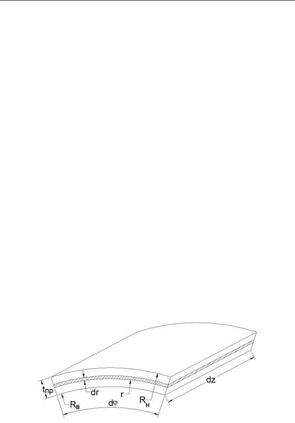
Further on another simplified model of the system “shell-soil” is investigated. The soil surrounding the shell is modelled by the approximated elastic layer (Fig. 1c). In order to account for the soil possibly sticking off the shell, the approximated elastic layer and the shell are joined with the contact GAP elements operating during compression as in the first case (Sсж = 107 n/m, Sр = 10-7 n/m). The material of the elastic layer is accepted to be orthotropic in the cylindrical system of coordinates with the same elasticity modulus in all the directions, the Poisson coefficients that all equal zero and the displacement modulus two units as low as for an isothropic material. This is due to seeking to approximate the behavior of the elastic layer as much as possible to the that of the elastic base, i.e. to reduce the effect of the displacement deformations in the elastic layer. Let us connect the approximated modulus of the elastic layer Eпр with the coefficient of the subbase of the elastic base K so that the elementary potential energies of the deformation layer and the base are dWсл dWос . We assume that the elastic layer (Fig. 4) operates during compression or tension only in a radial or circular direction and its outer surface is supported from displacements (wн = 0).

Fig. 4. Elementary segment of the elastic layer

12

The elementary potential energy of the deformation of the layer is given by the following formula

Strains and deformations in a radial and circular direction considering the accepted assumptions on a material are the following respectively:

Radial displacements of random points of the layer assuming that they change their thickness according to the linear law are calculated using the formula

The elementary potential energy of deformation of the base is determined using the formula

13

Russian journal of building construction and architecture

Equalling the expressions of the energy (8) and (9) we get

not considering deformations of the layer in the circular direction is given in [21]. It has no member containing a natural logarithm.

The elastic layer modelling the soil is approximated by eight-mode volumetric elements (Fig. 1c). The use of only one layer of the volumetric elements in this case is possible as the elastic characteristics of this layer are not real but approximated ones. Five calculations for different thicknesses of the elastic layer for the effect of the eigen weight of the shell for such supports are performed as in the previous sections. The outer surface of the elastic layer was accepted to be supported from all displacements. As a result, the components of the stressstrain of the shell are calculated. Maximum complete displacements wmax and maximum equivalent Mises strains in the internal вequiv and external нequiv fibers of the shell for different thicknesses of the elastic layer are listed in Table (columns “variant 3”). Note that for the other layer with the thickness of 0.08 m to 0.4 m (0.08Rв tпр 0.4Rв ) the calculated maximum displacements and strains in the shell were found to be quite close and consistent with the similar results obtained using the other models of the soil base. This is in agreement with the formula (11) and assumptions accepted as they were hypothesized.

Conclusions

As a result, the authors were able to develop the method considering one-sided contacts of the shell and the soil base to allow three models of the soil surrounding the shell to be compared: the Winkler-Fuss base, model of the elastic layer and volumetric massive. The accurate formula for the approximated elasticity modulus of the elastic layer is hypothesized. Let us sum up in the following way.

1. The results of the calculation of the system “shell-surrounding soil” obtained using three above models of soil are in good agreement qualitatively and quantitavely, which suggests

14

that the calculations and models were correct. Displacements, strains and deformations of the shell as well as areas where the soil sticks off are identical in all the cases.

2.The model of the approximated elastic layer should be applied unless there are finite elements in software that model the elastic base or the shape of the finite elements of the shell is regular. For the latter calculating actual stiffness of the GAP elements.

3.While choosing the thickness of the approximated elastic layer and using the formula (11) it should not be made too thick (tпр 0.4 0.5 Rв ).

4.In calculations we should avoid using mostly volumetric models of the massive of the soil with contact elements for considering the fact it might stick off the shell but due to complexity associated with such calculations it is acceptable to make use of the elastic base modelled using GAP elements as well as the model of the approximated elastic layer with extra contact elements.

References

1.Kositsyn S. B., Chan Suan Lin'. Chislennyy analiz napryazhenno –– deformirovannogo sostoyaniya ortogonal'no peresekayushchikhsya tsilindricheskikh obolochek bez ucheta i s uchetom ikh odnostoronnego vzaimodeystviya s okruzhayushchim massivom grunta [Numerical analysis of stress –– strain state orthogonal intersecting cylindrical shells with and without taking into account their unilateral interaction with the surrounding soil]. International Journal for Computational Civil and Structural Engineering, 2014, vol. 10, iss. 1, pp. 72––78.

2.Kleyn G. K. Raschet podzemnykh truboprovodov [Calculation of underground pipelines]. Moscow, Izdatel'stvo literatury po stroitel'stvu, 1969. 240 p.

3.Leont'ev N. N. [A practical method of calculation of thin-walled cylindrical pipe on an elastic Foundation]. Trudy Moskovskogo inzhenerno-stroitel'nogo instituta [Proc. of the Moscow Institute of civil engineering]. Moscow, 1957, pp. 47––69.

4.Prevo R. Raschet na prochnost' truboprovodov zalozhennykh v grunt [Strength calculation of pipelines laid in the ground]. Moscow, Stroyizdat Publ., 1964. 123 p.

5.Shaposhnikov N. N. [Calculation of circular tunnel linings in elastic Foundation characterized by the two ratios of bed]. Nauchnye trudy Moskovskogo instituta inzhenerov zheleznodorozhnogo transporta [Proc. of the Moscow Institute of railway transport engineers], 1961, iss. 131, pp. 296––305.

6.Shagivaleev K. F. Raschet zamknutoy tsilindricheskoy obolochki, zapolnennoy sypuchim materialom, na radial'nuyu nagruzku [The calculation of a closed cylindrical shell filled with loose material, radial load].

Izvestiya vuzov. Stroitel'stvo, 2003, no. 2, pp. 20––23.

7.Gabbasov R. F. K raschetu gibkikh trub na sovmestnoe deystvie vneshney nagruzki i vnutrennego davleniya s uchetom otpora grunta [To the calculation of flexible pipes for the joint action of external loads and internal pressure, given the resistance of the soil]. Gidrotekhnicheskoe stroitel'stvo, 1970, no. 10, pp. 17––19.

15